3Blue1Brown · Neural Networks and Deep Learning
The full 8-chapter neural network series, in order, each with my notes — from a single neuron to how transformers store facts.
 刁政欣8 videos8 notes
- 01
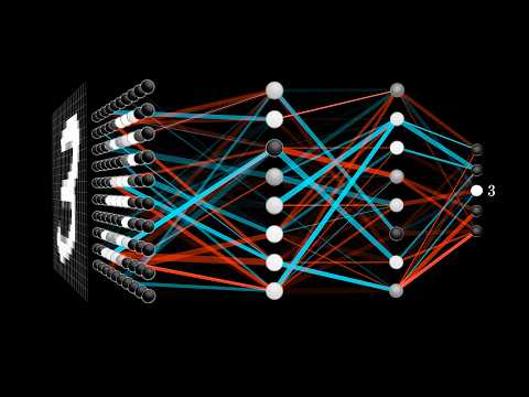 But what is a neural network? | Deep learning chapter 1
Learned3Blue1Brown
This video introduces the fundamental structure of a neural network, using the example of recognizing handwritten digits. It explains how neurons, weights, biases, and activation functions work together to process information, setting the stage for a follow-up on learning algorithms.
One line: A neural network is just a big function: 784 pixel values go in, 10 digit scores come out, and everything in between is weights and biases.
- Input layer = 784 neurons (28×28 pixels), two hidden layers of 16, output layer of 10. Each neuron holds a single number between 0 and 1, its "activation".
- Every connection has a weight, every neuron a bias. Weighted sum + bias, squished by a sigmoid (0 to 1), decides how strongly the next neuron fires.
- That little network already has about 13,000 knobs. "Learning" means finding good values for all of them.
- The hope is that layers build abstraction: pixels → edges → loops and lines → digits. Whether the trained network actually does that is a question for the next video.
My take: Stop thinking of "neurons" as biology. A neuron is a number, a layer is a vector, and the whole network is matrix multiplication plus a nonlinearity. Sigmoid is the textbook version; ReLU is what people actually use now.
- 02
 Gradient descent, how neural networks learn | Deep Learning Chapter 2
Learned3Blue1Brown
This video explains how neural networks learn by minimizing a cost function through gradient descent. It also analyzes the hidden layers' learned features and discusses limitations of the simple network, leading to a discussion on modern research.
One line: Learning = finding the weights and biases that make the cost function as small as possible, by walking downhill along the negative gradient.
- Cost of one example: sum of squared differences between the output and what it should have been. Average that over all 13,000-ish parameters' worth of training data and you get one number to minimize.
- The gradient tells you the steepest uphill direction; step the other way, repeat. The size of each gradient component says which weights matter most.
- On MNIST this gets ~96% after training, but the hidden layers don't learn clean edges and loops. They learn loose, blurry patterns.
- The network is confidently wrong on random noise: it always outputs some digit, because it was never shown "not a digit".
My take: The local minimum is not necessarily the global one, and that's fine in practice. The bigger lesson is that "it works" and "it learned what we hoped" are two different claims.
- 03
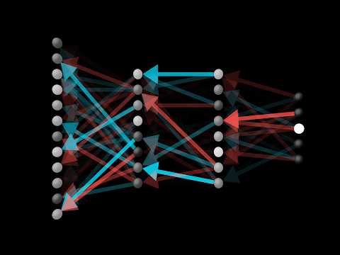 Backpropagation, intuitively | Deep Learning Chapter 3
Learned3Blue1Brown
This video explains backpropagation, the algorithm used to compute the gradient of a cost function in neural networks. It provides an intuitive walkthrough of how a single training example influences weight and bias adjustments, then discusses practical implementation like stochastic gradient descent. Viewers gain a clear conceptual understanding of the mechanics behind backpropagation without diving into calculus.
One line: Backpropagation is how you compute the gradient: figure out how each output wants to change, then push that wish backwards through the layers.
- For one training example, look at the output layer: raise the activation of the correct digit, lower the others. That's a list of desired nudges.
- Three ways to change an activation: change the bias, change the weights (bigger effect from neurons that fire strongly), or change the previous layer's activations.
- Add up the nudges every output neuron wants for the previous layer, and you have desired changes for that layer. Repeat backwards. That's the "propagation".
- Averaging these nudges over all training examples is too slow, so use mini-batches (say 100) for a noisy but fast estimate. That's stochastic gradient descent.
My take: Backprop is not mysterious; it's bookkeeping. The intuition "neurons that fire together wire together" comes straight from the weight update being proportional to the previous activation.
- 04
 Backpropagation calculus | Deep Learning Chapter 4
Learned3Blue1Brown
This video formally presents the calculus behind the backpropagation algorithm for neural networks. It shows how the chain rule is applied to compute the sensitivity of the cost function to weights and biases, starting with a simple single-neuron network and extending to multi-neuron layers.
One line: The math behind chapter 3. Everything reduces to the chain rule applied to one path: weight → z → activation → cost.
- Set up a chain of single neurons. Define z = w·a_prev + b, a = σ(z), C = (a − y)².
- ∂C/∂w = ∂z/∂w · ∂a/∂z · ∂C/∂a = a_prev · σ'(z) · 2(a − y). Three ratios multiplied together, each one simple.
- Same trick for the bias (∂z/∂b = 1) and for the previous activation (∂z/∂a_prev = w), which is what lets you keep walking backwards.
- With many neurons per layer, nothing changes except indices: sum over the paths through which a_prev influences the cost.
My take: Once you've seen the full-derivative formula, the tree of dependencies is the whole algorithm. Writing it out for a single neuron chain was the thing that finally made it click.
- 05
 Large Language Models explained briefly
Learned3Blue1Brown
This video explains how large language models (LLMs) work, from next-word prediction to training on massive datasets and the transformer architecture. It highlights the role of attention and feed-forward networks, and touches on reinforcement learning with human feedback.
One line: A large language model is a function that predicts the next word, made useful by staggering scale and some training tricks.
- Feed it text, get a probability for every possible next word. Sample, append, repeat, and you get a chatbot.
- Pre-training on internet-scale text tunes hundreds of billions of parameters. Done by one human at a billion ops per second, it'd take over 100 million years.
- Transformers (2017) read all the text in parallel rather than word by word, which is what lets training spread across GPUs.
- After pre-training, reinforcement learning from human feedback nudges the model toward answers people actually rate as helpful.
My take: "Emergent behavior" here just means nobody hand-designed the reasoning; it fell out of next-word prediction at scale. The parameters were tuned, not written.
- 06
 Transformers, the tech behind LLMs | Deep Learning Chapter 5
Learned3Blue1Brown
This video provides a visually-driven introduction to transformers, the neural network architecture behind large language models like GPT. It explains the flow of data through a transformer, covering tokenization, embeddings, attention blocks, and the final prediction, while also reviewing key background concepts and parameter counts for GPT-3.
One line: Data flow through a transformer: text → tokens → embedding vectors → attention and MLP blocks, over and over → one probability distribution for the next token.
- Tokenize the input; each token becomes a vector from an embedding table (GPT-3: 12,288 dimensions, 50k vocabulary). Similar meanings point in similar directions.
- Dot products measure alignment between vectors. That's the primitive that attention is built on.
- Attention lets tokens talk to each other; MLP blocks process each vector on its own. Alternate them many times.
- The last vector goes through an "unembedding" matrix and a softmax (with a temperature) to become next-token probabilities. GPT-3 has 175 billion parameters in total.
My take: The diagram to keep in your head is a stack of vectors flowing left to right, being nudged at every block. Everything else is details about how the nudges are computed.
- 07
 Attention in transformers, step-by-step | Deep Learning Chapter 6
Learned3Blue1Brown
This video explains the attention mechanism in transformer models, covering how tokens are embedded, how queries, keys, and values are used to compute attention patterns, and how multiple attention heads work in parallel to refine embeddings. The viewer learns the fundamental computations and parameter counts behind attention in models like GPT-3.
One line: Attention is how a token's embedding gets updated by context: "a fluffy blue creature" moves the vector for "creature" toward fluffy and blue.
- Each token produces a query (what am I looking for?) and a key (what do I offer?). Query·key dot products, softmaxed per column, give the attention pattern.
- Mask out future tokens (set to −∞ before softmax) so the model can't peek ahead during training.
- Each token also produces a value; the weighted sum of values, per the attention pattern, is what gets added to the embedding.
- One head in GPT-3 is about 6.3 million parameters; 96 heads per layer, 96 layers, roughly 58 billion parameters in attention alone.
My take: "Multi-head" is just running many of these in parallel so different heads can capture different kinds of relationships: adjectives, subjects, references. The value matrix is factored into two small matrices for efficiency, which I'd missed on first watch.
- 08
 How might LLMs store facts | Deep Learning Chapter 7
Learned3Blue1Brown
This video explains how facts are stored in large language models by focusing on the multilayer perceptron (MLP) blocks within a transformer. It walks through the computational steps of an MLP with a concrete toy example of storing 'Michael Jordan plays basketball,' then reflects on where parameters live and the concept of superposition.
One line: Facts like "Michael Jordan plays basketball" live in the MLP blocks, which hold about two thirds of a transformer's parameters.
- An MLP block: multiply by a big up-projection matrix, add a bias, apply ReLU, multiply by a down-projection, add the result back to the vector. Same operation on every token, independently.
- With ReLU, a neuron can act as an AND gate: it only fires when both "Michael" and "Jordan" directions are present, and then the down-projection adds the "basketball" direction.
- GPT-3: each MLP block has about 1.2 billion parameters; across 96 layers that's most of the model.
- Superposition: in high dimensions you can fit far more nearly perpendicular directions than dimensions, so a model can store many more features than its vector size suggests. Good for capacity, bad for interpretability.
My take: The toy example is idealized, but it makes the mechanism concrete. The real surprise is superposition: features aren't neurons, they're directions, and there are many more of them than you'd think.